Number Square Project
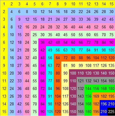
 This project will result in you making a square that you can use to multiply two numbers together.
Open a new Excel Spreadsheet and save it as 'NumberSquare'.
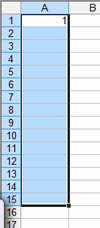
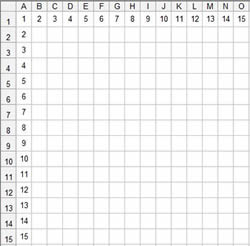
Put the number '1' in cell A1. Select that cell using the left mouse button - hold the button down and sweep through the column to row 15 - you will see the cells liight up in blue as you do this - see the graphic on the right.
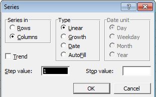
From the top menu bar select 'Edit' - 'cloumn' - 'Fill' - 'Series'
A new window will open. It gives you the choice of what 'series of numbers' you wish to fill down the column. We need the numbers to increase by a 'step of 1' each time so make the step '1' and then press OK.
The numbers 1 to 15 will fill automatically.
Do the same for the row from A1 to O1 - filling in numbers from 1 to 15 along the top row.
Making the cells into squares - with centred numbers
The width of the columns is too great and the height of the rows is too small.
Highlight all of the columns by selecting the letters A to O above your grid of cells.They will light up blue.
On the top menu bar select 'Format' - 'Column' - 'Width' and a little box will appear. Put the number 3 in that box and the column width will reduce.
Do the same for the rows... but you need to make the row height 20.
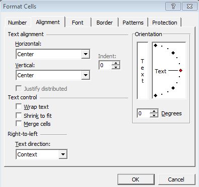
Highlight your square and then go to 'Format' again. You need to format the cells. Make the text position central both horizontally and vertically.
Your square will then look like this:
Inserting the formulae
Column B needs to house the two times table.
The A cells in turn need to be multiplied by the contents of cell B1. Cell B1 needs to be the cell in each of the formulae... the A cells need to change as you go down the column.
When you 'fill down' a formula Excel automatically makes the adresses follow a sequence. This is relative cell referencing. The cell it puts into the new formula is the cell that has the same distance on the grid as the one you are copying from.For example if you are adding the adjascent cell the adjascent cell will be referenced in the fill down...
To stop a cell address being changed you have to insert a dollar sign before the letter and number in the address. This makes it an absolute cell reference.
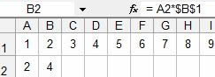 The formula we need in cell B2 is therefore:
= A2*$B$1
This means that the contents of A2 has to be multiplied (*) by the contents of B1.
The formula window above the grid shows the formula - the cell itself shows the contents.
Highlight that B2 cell and holding down on the left button pull down highlighting the cells down the column. The choose to fill down - Edit - Fill - Down. and the whole column will fill with the two times table.
Repeat this for the other columns:
= A2*$C$1 and =A2*$D$1 etc. in the headers.
You should then have a tables square... you can then colour in the columns and rows as you wish.
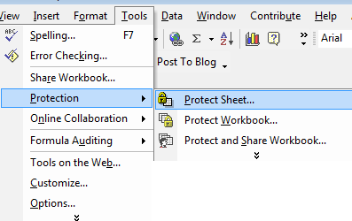
Protect your work
If you want to be sure that no one can enter numbers into your square and mess it up you need to protect your sheet. The option is in the 'Tools' section.
You can add a password - but remember it - otherwise you will not be able to amend it ever again!