Lesson 3: Making a Simple Spreadsheet
Now we are going to get the spreadsheet to work out the average percentage for each test and the average percentage for each student. We will also get the computer to pick out the maximum and minimum scores on the test to work out the spread of marks. So, let's get started!
Open up your spreadsheet Potions_NEWT and save it as Potions_NEWT2. (It is always a good idea not to lose an original document state. If you make a mess of things you may want to go back to it!). Computer programs need you to express commands in a particular way - you have to get the syntax correct. Syntax is a linguistic term - it relates to the correct grammatical ordering of words within a sentence. Computers 'speak' a very strict language - you have to get it right! One of the most useful things about Excel is that it can 'do the math' for you. You enter an equation formula into a cell and it displays the answer to that equation in the cell for you. Here is a link to list of useful calculation formulae for Excel. Take a good look at them. We need to use them to help Professor Snape analyse the results of his NEWT students. You have to be very careful to include parentheses and colons where they are indicated... missing them out will mean that the computer program will not understand your formula!
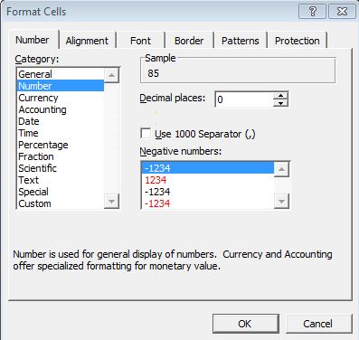
Finding the average Add another column to your spreadsheet. Call it 'Average'. In that column we are going to find the average mark that each student got for the three tests. Fore Paige the formula will be: =AVERAGE(C2:E2) Type in =AVERAGE( and then click on her result for the first test - add a colon to the formula and then click on the result for her last test. All three test marks will be selected by the computer. Now close off the formula with a closing bracket and voila - her average make appears! It is 85.3333333 - that is far too many figures. We need to format the number. Select the cell - click on 'Format' and select 'Cell' then 'Number'. Change the number of decimal places to zero and press 'Okay'
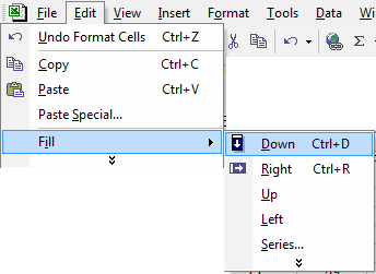
We now have 85 as the average - that is better. We could do the same for each of the students - but there is a timesaveing way to do that. Select Paiges average value and hold down the mouse button as you drag down to highlight the average value cells for all of the students. Release the button and then go to Edit in the main menu bar - chosse fill - then down... and 'hey presto!' the computer will calculate averages for all of the students and put them to zero decimal places. Isn't that neat!?
I now want you to work out the average for each test - and the Max and Min values for each test. Take a look at my spreadsheet and see if you can do the same. You will need to look at the formula page to find out the syntax for the formulae you will need. |
|

Custom Search
 Last lesson we set up a spreadsheet for the good Professor