Lesson 2: Making a Simple SpreadsheetWe are going to make a simple spreadsheet of the type that a teacher might use to keep record of test scores. Here is a copy of the results of the last three tests taken by Professor Snape's Advanced Potions Class
When you click on each of the scrolls you will open a tab with a magnified image of each scroll so that you can read the data easily.
We will use the spreadsheet to organsise the names into alphabetical order. In the next lesson we are going to get the spreadsheet to work out the average percentage for each test and the average percentage for each student. So, let's get started!
Open a new spreadsheet and call it Potions_NEWT Now take a look at the first scroll of data. We have three types of data there - the name of the test, the names of the students and the marks the students attained in the test. If we look at the next two scrolls we see a similar set of data. The common data is the names of the students - that is the same in all three scrolls - as they are his 'NEWT' class. We have to think how best to lay the data out - with practice you will do this without thinking about it very much - but at this stage lets put thought and planning into the task!
We will put the names in the first two columns - forename then surname. So head those columns up as Forename and Surname. To make the heading stand out make it bold. Select the cells A1 and B1 and then click the B for bold in the header. Then using the first scroll type in the student names.You will find that you have to adjust the width of the columns to fit in the names. Adjusting column width
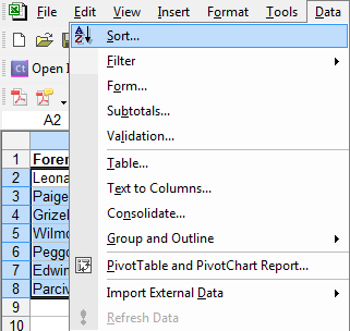
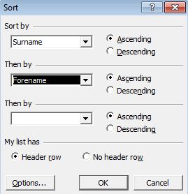
We now need to sort the names into alphabetical order. We want the A and B data to stay together, we therefore have to select ALL of the name block. Sorting data into alphabetical order
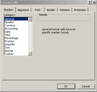
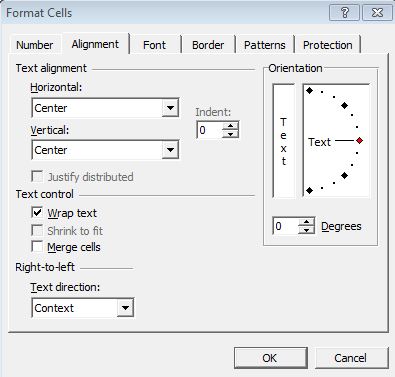
Now let's head up the next three columns with the names of the three tests. These are quite long, but the data we are entering is only a few digits in size. We will have to wrap the text - make the text occupy several lines within the cell. The problem we will then encounter is that the row will not be high enough for us to see all of the text. We will therefore have to adjust the row height so that all of the name is visible in a narrow column. Wrapping Text
Adjusting row height
Beneath each test name put the result that each pupil obtained for that particular test. Select them and centre to data. Now save your spreadsheet - you will need it for the next lesson! Here is a copy of my spreadsheet: Click here to download
|
|

Custom Search
 Our task is to help the good professor assess the progress of his students by putting the data from the scrolls into an Excel Spreadsheet.